The dynamic range of an audio passage is the ratio of the loudest signal to the quietest signal. For signal processors the magnitude of the power supply voltages restricts the maximum output signal and the noise floor determines the minimum output signal.
Professional-grade signal processing equipment can output maximum levels of +26 dBu, with the best noise floors being down around -94 dBu. This gives a dynamic range of 120 dB -- an impressive number coinciding nicely with the 120 dB dynamic range of normal human hearing. The invention of dynamics processors came about because this extraordinary range is too great to work with.
Dynamics processors alter an audio signal based upon its frequency content and amplitude level; hence the term "dynamics" since the processing is program dependent and ever changing. The four most common dynamics effects are compressors, limiters, gates and expanders. After these come a whole slew of special purpose processors: AGC units, duckers, de-essers, levelers, feedback suppressors, exciters and enhancers. No matter what the name, all are in the business of automatically controlling the volume, or dynamics of sound -- just like your hand on the volume fader.
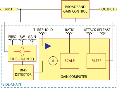
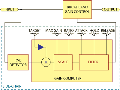
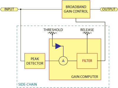
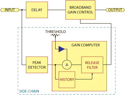
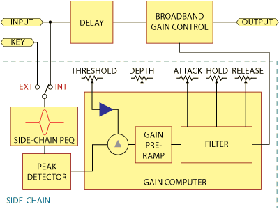
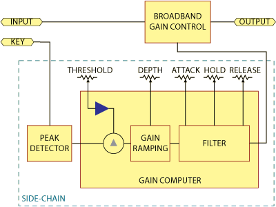
All dynamics processors have the common structure shown in Figure 1: a gain control element in the main signal path and a side-chain containing a detector and gain computer. The detector may sample the signal before the gain control element or after it, but for simplicity we show it before.
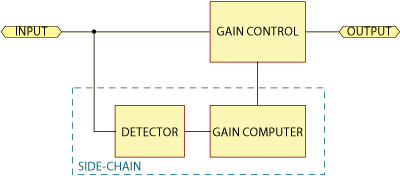
The signal path is the route the main audio takes through the unit. Typically, the signal goes through the input circuits, on to the gain control device and then exits through the output circuits (or the digital equivalent of this path). Thus, the signal chain goes through the "volume control" in the "hand on a control" analogy.
The side-chain is the hand that controls the volume. Side-chain circuitry examines the input signal (or a separate Key Input) and issues a control voltage to adjust the gain of the signal path. In addition, a side-chain loop allows patching in filters, EQ or other processors to this path. More on this and a description of the type of side-chain controls later.
Some dynamics processors make the side-chain control voltage available for connecting to a neighboring unit, or to tie internal channels together. Slaving or linking dynamics processors causes the units to operate simultaneously when only one unit or channel exceeds the threshold setting. This feature preserves stable stereo imaging and spectral balance.
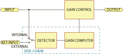
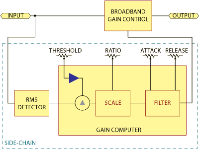
All dynamics processors carry out gain control as a function of side-chain level. Some use the internal signal as shown in Figure 1 and some use an external or Key Input as shown in Figure 2.
The only difference between a compressor, limiter, AGC, de-esser, ducker, or gate, is the type of side-chain detector, the gain computer attributes and the type of gain control element used.
The introduction of DSP (digital signal processing) dramatically changed the implementation of dynamics processors. In traditional analog designs, there is no practical means of "looking ahead" or statistically analyzing the content of a signal, instead requiring a function to respond to events that have already occurred. The supporting circuitry for filtering and dynamic control of attack and release is complex and expensive with limited accuracy.
At the heart of analog designs are gain control elements, usually voltage-controlled amplifiers, or voltage-controlled attenuators (both abbreviated VCA), with these typical specifications:
Certainly respectable numbers, but digital designs can do better. The most significant advantages are the ability to analyze a signal before it is processed and statistically analyze recent history. These abilities allow a wide range of new topologies offering superior performance; some of which appear later in this note. The incremental cost of a single function implemented in DSP is very small, resulting in significant cost reduction when requiring multiple functions. Digital signal processing offers both greater accuracy and reduced cost.
Compressors reduce (compress) the dynamic range of the signal passing through them; they turn down the loudest signals dynamically. A compressor begins turning down the signal by an amount set by the ratio control when the input signal exceeds the level set by the threshold control. A compressor changes the dynamics for purposes of aesthetics, intelligibility, recording or broadcast limitations.
For instance, an input dynamic range of 110 dB might pass through a compressor and exit with a new dynamic range of 70 dB. This clever bit of skullduggery is done in analog designs using a VCA whose gain is determined by a control voltage derived from the input signal (other schemes exist but VCAs dominate). Digital designs use complex mathematical algorithms optimized for music and speech signal dynamics. Before compressors, a human did this at the mixing board and we called it gain riding.
The difficulty that sound systems have handling the full audio range dictates dynamic range reduction. If you turn it up as loud as you want for the average signals, then along come these huge musical peaks, which are vital to the punch and drama of the music, yet are way too large for the power amps and loudspeakers to handle. Either the power amplifiers clip, or the loudspeakers bottom out, or both — and the system sounds terrible. Or going the other way, if you set the system gain to prevent these overload occurrences, then when things get nice and quiet, and the vocals drop real low, nobody can hear a thing.
To fix this, you need a compressor.
Using it is quite simple: Set a threshold point, above which everything will be turned down a certain amount and then select a ratio defining just how much a "certain amount" is, in dB. All audio below the threshold point is unaffected and all audio above this point is compressed by the ratio amount. The earlier example of reducing 110 dB to 70 dB requires a ratio setting of 1.6:1 (110/70 = 1.6).
The key to understanding compressors is always to think in terms of increasing level changes in dB above the threshold point. A compressor makes these increases smaller. From the example, for every 1.6 dB increase above the threshold point the output only increases 1 dB. In this regard, compressors make loud sounds quieter. If the sound gets louder by 1.6 dB and the output only increases by 1 dB, then the loud sound is now quieter.
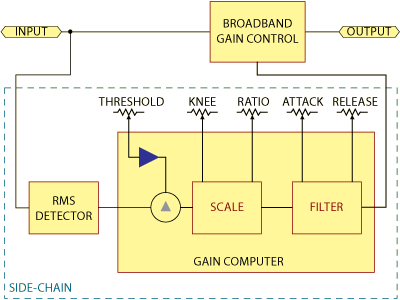
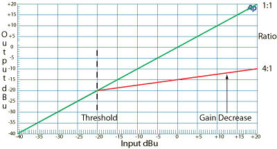
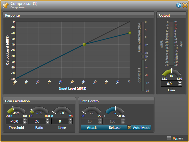
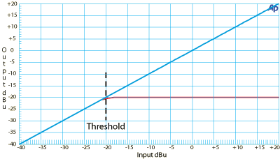
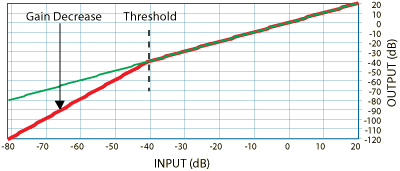
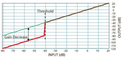
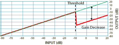
Broadband compression is the simplest form of compression, where all frequencies are compressed equally and the side-chain is equally sensitive to all frequencies. An rms detector is typically used and the basic gain computer side-chain controls are threshold, ratio, attack and release as shown in Figure 3a. The response of an above-threshold compressor with a threshold of -20 dB and a ratio of 4:1 is shown in Figure 3b. Some compressors operate above and below threshold as shown later in the Automatic Gain Control (AGC) example and in the Appendix.
Compression is available in several forms. As explained earlier the basics are the same for all types: a side-chain level is compared to a threshold and a gain computer uses the difference between the threshold and the side-chain level in combination with the side-chain control settings to determine the gain. Each of the compression techniques that follow, evolved to satisfy a specific need.
A number of parameters govern side-chain activity, but the four primarily ones are Threshold, Ratio, Attack and Release. Some dynamics controllers offer front-panel adjustment of these parameters, or software control, while others auto-set them at optimum values.
Threshold and Ratio have unambiguous definitions:
Like crossing through a doorway, this is the beginning point of gain adjustment. When the input signal is below the threshold for compressors, or above the threshold for expanders, a dynamics processor acts like a piece of wire. Above the threshold, the side-chain asserts itself and reduces the volume (or the other way around for an expander). A workable range for compressors is -40 dBu to +20 dBu. A good expander extends the range to -60 dBu for low-level signals.
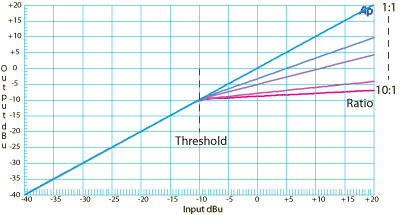
Once the signal exceeds the threshold setting, just how much the volume changes depends on the ratio setting. A straight wire has a ratio of 1:1 -- the output tracks the input -- a 2 dB change at the input produces a 2 dB change at the output.
A severe ratio is 10:1. For a 10:1 ratio, a 10 dB blast at the input changes only 1 dB at the output -- this represents heavy processing. Kinder, gentler ratios are in the 2:1 to 3:1 range.
Figure 4 shows the normal ranges for ratio controls of 1:1 to 10:1. If provided, the lower limit of 1:1 is for bypassing.
Sometimes referred to as "make-up gain" in compressors, this controls the desired output level with compression active. The preferred range for professional applications is ±12 dB with a center-detent 0-dB unity gain position. Gain can be done in the main signal path, or in the side-chain as control offset.
Unfortunately precise definitions for the terms attack and release do not exist due to a lack of industry standards. Moreover, manufacturers make this worst by not explaining how they define the terms. Most don't, they just list a range of settings, leaving the user to guess if the time shown represents how long it takes to get to the end of the gain change, or to the middle, or the 3-dB point, or what -- caveat emptor.
Defines how quickly the function responds to an increase in side-chain input level above the threshold. For compressors and AGC, this defines how quickly the gain is turned down. For gates and expanders, this defines how quickly the gain is turned up.
Because increasing time has a diminishing effect on gain for compressors, it is practical to specify attack as the time required for gain to settle to a defined percent of final value. Typical are 86% or 95% of the final value.
Attack times for compressors generally range between 25 ms and 500 ms.
For expanders (with ducking & gate features) this range changes to 0 ms ("instantaneous" attack, relative to any DSP or look-ahead delay for digital processors) to 250 ms (since longer attack times are not necessary).
In expand mode, attack time determines the rate of gain increase as the control signal moves toward or above the set threshold.
In gate mode, attack time determines how quickly the gate opens once the control signal exceeds the threshold setting.
In ducker mode, attack time determines how quickly the signal is reduced as the control signal exceeds the threshold setting.
Defines how quickly the function responds to a decrease in side-chain input level below the threshold. For compressors and AGC, this defines how quickly the gain is turned back up once these processes have stopped. For gates and expanders, this defines how quickly the gain is turned down. Release is typically defined by an RC (resistor-capacitor) time constant in the log domain, resulting in a constant dB per second gain change at the output. Because the dB per second is constant, release can be specified directly in dB/second or as the time required for a 10 dB change (typically a 10 dB step).
It is important to understand the difference between release rate -- as determined by this control -- and release time. There is no industry standard and different manufacturers define this control differently.
Rane defines this control, in a compressor for example, as how long it takes for the gain to change by 10 dB, not how long it takes to return to unity gain (no gain reduction).
To calculate the actual release time requires a little math: Release Time = (Gain Reduction x Release Setting) / 10 dB
Example: with the release control set to 1 sec, when a signal with 5 dB of gain reduction presently applied suddenly drops below threshold, the release time is:
(5 dB x 1 sec) / 10 dB = 0.5 sec.
Typical compressor and expander release settings are between 25 ms and 2 seconds.
In gate mode, the release time determines how quickly the gate closes as the control signal drops below the threshold setting.
In expand mode, the release time determines how quickly the signal is turned down as the control signal moves below the set threshold.
In duck mode, the release time determines how quickly the signal is ramped up when the control signal drops below the threshold setting.
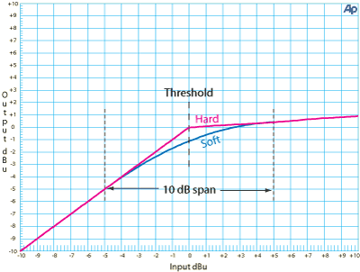
Unique to compressors, this function controls the action at the threshold point. Hard knee does nothing until the signal exceeds the threshold point, and then applies full compression.
Use of a soft knee significantly reduces distortion caused by abrupt transitions from unity gain to a compressed signal. An accurate soft knee response is difficult to achieve using analog methods. Digital implementations allow locating the center of the knee exactly at the threshold with a mathematical function defining a smooth transitioning from unity gain to the specified ratio. Note in Figure 5 that a proper soft knee response does not alter the ultimate gain reduction achieved above the knee, which commonly occurs in analog designs. A soft knee is defined by the "span." The span defines how many dB below the threshold compression begins and how many dB above the threshold compression reaches the specified ratio.
Soft knee begins applying a small amount of compression just before the threshold point is reached, continues increasing compression through the threshold point and beyond, finally applying full compression to the highest level signals. Depending on the application and source material, soft knee settings sound more natural. However for maximum loudness before compression (equipment protection for instance) use hard knee settings.
This chapter explores very useful variations on the basic compressor technology. Adding a parametric equalizer section in the side-chain creates a frequency sensitive compressor; using a crossover allows split-band compression; putting a tracking filter into the main signal path and side-chain gives you a dynamic EQ; comparing broadband and bandpass energies produces a relative threshold dynamic EQ, which makes a terrific de-esser; while other clever additions solve the problems of automatic gain control and peak limiting. Here are the details:
Frequency sensitive compression is broadband compression as described above with the addition of side-chain equalization to make the detector more or less sensitive to certain frequencies. The basic topology is shown in Figure 6. Side-chain equalization may take the form of a parametric filter (with variable boost, cut and bandwidth), high-cut filter, low-cut filter or all three. In some cases, multiple parametric filters or a multiband graphic are used in the side-chain. If the amplitude of a frequency in the side-chain is reduced, the broadband compressor is less sensitive to it. If the amplitude of a frequency is boosted in the side-chain, the broadband compressor is more sensitive to it.
Split-band Compression divides the incoming signal into two or more frequency bands as shown in Figure 7. Each band has its own side-chain detector and gain reduction is applied equally to all frequencies in the passband. After dynamics processing, the individual bands are re-combined into one signal. The handling of in-band signals is the same as for the general-case compressor shown above.
This configuration is easily done with Rane's Halogen software and HAL processors as shown in Figure 8. This quickly expands into three, four or more frequency bands as required. Moreover, adding side-chain EQ and filters is just a drag and drop away.
Dynamic EQ differs from the forms of compression listed above in that it dynamically controls the boost/cut of a parametric filter rather than broadband frequency gain. The basic dynamic EQ uses a bandpass filter in the side-chain with variable center frequency and bandwidth. The side-chain detector is sensitive only to the passband frequencies. A parametric filter with matching bandwidth and center frequency is placed in the main signal path and the boost/cut of the filter is controlled the same way a broadband compressor boosts or cuts broadband gain. The basic topology is shown in Figure 9.
See the Application section in Part II for the many creative uses of Dynamic EQ.
Relative Threshold Dynamic EQ is a special form of dynamic EQ where the rms level of the bandpass signal in the side-chain is compared to the rms level of the broadband signal. The difference between the bandpass and broadband levels is compared to the threshold rather than the absolute rms value of the bandpass signal. The advantage of this type of dynamic EQ is that the relative amplitude of a band of frequencies, as compared to the broadband level, is maintained regardless of broadband amplitude. The typical topology is shown in Figure 10.
De-essing limits or controls the sibilant content of speech. Sibilance produces a hissing sound. English sibilant speech sounds are (s), (sh), (z), or (zh). De-essing is often confused as a type of dynamics processor. It's actually a specific application that is accomplished using many different types of dynamics processors. And contrary to popular belief, successful de-essing is not as simple as placing a bandpass or treble-boost filter in the side-chain and calling it done. Frequency Sensitive Compression, Split-Band Compression, Dynamic EQ and Relative Threshold Dynamic EQ are all used for de-essing.
True de-essing involves comparing the relative difference between the troublesome sibilants and the overall broadband signal, then setting a threshold based on this difference, therefore it is our experience that Relative Threshold Dynamic EQ (as described above) is the best dynamics processor for this task as it is able to maintain proper sibilant to non-sibilant balance regardless of level.
A good de-esser looks at the average level of the broadband signal (20 Hz to 20 kHz) and compares it to the average level of a bandpass filter in the side-chain. The threshold setting defines the relative threshold, or difference, between broadband and bandpass levels, which result in compression of sibilants. Because de-essing depends on the ratio of sibilant to broadband signal levels, it is not affected by the absolute signal level, allowing the de-esser to maintain the correct ratio of broadband to sibilant material regardless of signal level, as shown in Figure 11.
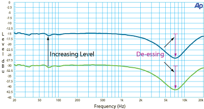
This means that the de-essing performance is consistent and predictable, regardless of how loud or quiet the singer/talker is. Taming sibilance when the talker is quiet is just as important as when the talker is at a fevered pitch.
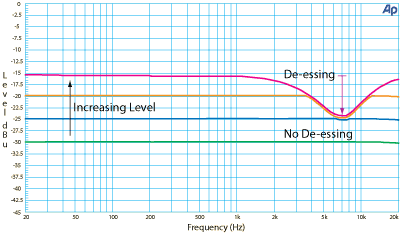
Figure 12 shows what happens using a primitive de-esser with a side-chain EQ. Sibilance during loud passages is attenuated, but there is no gain reduction during quiet passages, even though there may still be a significant amount of "sss" in the person's voice. For a given threshold, this often results in an overly aggressive effect during the loud choruses, and a completely ineffective result during the hissy, whispered verses.
Automatic Gain Control (AGC), also known as Automatic Level Control (ALC), is a specialized form of compression. It is a circuit or algorithm that varies gain as a function of the input signal amplitude. Commonly found in pro audio applications where you want to automatically adjust the gain of different sound sources in order to maintain a constant loudness level at the output. One of the most common applications is for speech. Another example, on better DJ mixers the gain adjusts automatically when the DJ switches sources between records, CD, or MP3 files. Not only do signal levels differ greatly between different source technologies but also between any two examples of the same technology, e.g., between CDs, or between MP3 files, etc.
AGC is more similar to older compressor designs which compressed a signal about a threshold value (see Appendix). In these designs, gain was reduced for signals above the threshold and increased for signals below the threshold. One of the problems encountered with this type of compressor is the possibility of very high gain at low signal levels.
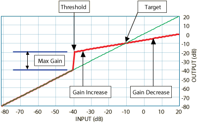
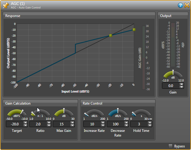
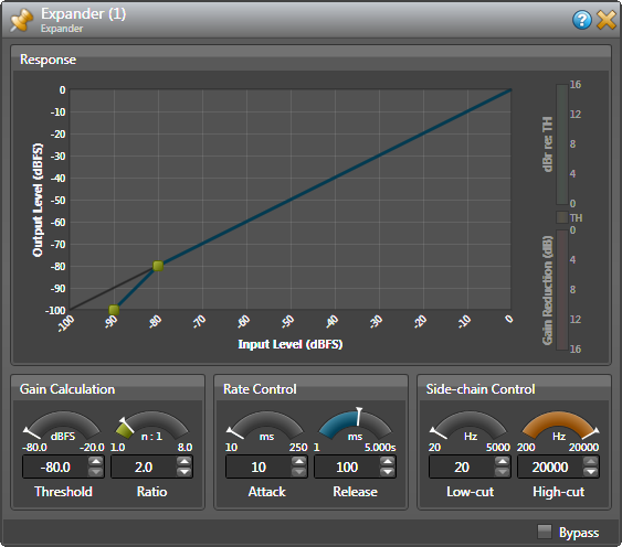
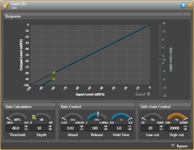
A typical modern AGC implementation is shown in Figure 13a. Note that the traditional threshold control is now labeled target. The target is the desired, nominal level. As with early compressors, gain is reduced for signals above the target and increased for signals below the target as shown in Figure 13b. Note the gain is unity (input = output) at the target. The threshold is defined as the level below which the AGC circuit will not increase the gain. Note the gain is unity (input = output) below the threshold. The implementation shown in Figure 13a indirectly determines the threshold for given maximum gain and ratio settings. Other implementations exist, but the basics are the same. The hold parameter determines how long the above threshold gain is held in the absence of a signal. For speech, this feature allows the correct gain to be held during pauses. Figure 13c shows the control screen for Rane's Halogen AGC module.
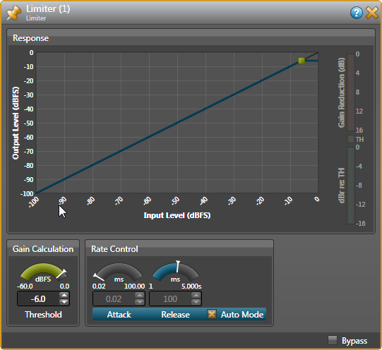
As expected, the basic topology of the limiter is similar to that of the compressor. Unlike the compressor, the limiter must ensure that a signal never exceeds the set threshold. This requires the use of a peak responding detector and a fixed ratio of infinity:1. Figure 14a illustrates the basic topology. The response of a limiter with a threshold of -20 dB is shown in Figure 14b.
While the basic operation of a limiter is straightforward, coaxing one to sound good is challenging. Abrupt limiting causes significant alteration of the sound and determining the best release rate for a particular signal is problematic. Digital signal processing enables two additions to the basic topology which go a long way toward resolving these issues. First, adding delay in the main signal path allows the side-chain to "see what's coming", and start to respond prior to the threshold actually being reached. The result is a softer leading edge resulting in a more natural sound. Second, looking at recent history gives the system knowledge of where the signal has been and where it is likely to go. With this knowledge, the best release rate is set dynamically. Figure 15 illustrates the topology.
Primarily used for preventing equipment, media, and transmitter overloads, a peak limiter is to a compressor as a noise gate is to an expander (more on this later).
The most useful dynamics processor designs incorporate a separate peak limiter function independent of the compressor. A separate peak limiter frees the compressor from the task of clamping wild excursions. The peak limiter plays level-police while the compressor persuades more gently.
Expanders complement compressors by increasing (expanding) the dynamic range of the signal passing through it, i.e., an expander is a compressor running in reverse. For example, a compressed input dynamic range of 70 dB might pass through an expander and exit with a new expanded dynamic range of 110 dB.
As shown in Figure 16a, the topology for an expander looks just like a compressor. The difference is what the gain computer is directed to do with the difference between the threshold and the detected signal level. Unlike a compressor, the expander reduces gain for signals below the threshold. The ratio still defines output change verses input change as shown in Figure 16b. In this example, the ratio is 2:1. For every 10 dB of reduction in input signal, the output is reduced by 20 dB. Operating in this manner, they make the quiet parts quieter. A compressor keeps the loud parts from getting too loud, an expander makes the quiet parts quieter.
The term downward expander (or downward expansion) evolved to describe this type of application. The most common use is noise reduction. For example, say, an expander's threshold level is set just below the quietest recorded vocal level and the ratio control is set for 2:1. What happens is this: when the vocals stop, the signal level drops below the set point down to the noise floor. This is a step decrease from the smallest signal level down to the noise floor. If that step change is, say, -10 dB, then the expander's output attenuates 20 dB (due to the 2:1 ratio, a 10 dB decrease becomes a 20 dB decrease), thus resulting in a noise reduction improvement of 10 dB. It is now 10 dB quieter than without the expander.
A live sound use for an expander is to reduce stage noise between passages for a quiet vocalist.
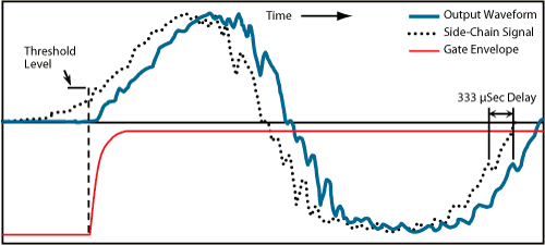
A gate is to an expander, as a limiter is to a compressor. Like an expander, gain is reduced below the threshold. Like a limiter, a gate must respond very quickly to changes in level, dictating the use of a peak detector in the side-chain. Unlike an expander, a gate uses a fixed ratio of infinity:1 and a variable depth as shown in Figure 17a. A gate is typically used to remove background noise between louder sounds. The common topology is illustrated in Figure 17a. Almost all gates provide side-chain equalization and external Key Input. A good gate is able to "look-ahead" by delaying the main signal a small amount. The best gate combines look-ahead with pre-ramping.
Provided by professional gates, with a typical range of 0 to 3 seconds. The hold time determines how long the gate remains open after the control signal drops below the threshold setting.
Provided on all gates, this control has a typical range of 0 to -80 dB. The depth control determines how many dB the signal is attenuated when the control signal is at or below the threshold setting.
Gates find use in live sound to reduce crosstalk (bleed) from adjacent microphones, to keep toms from ringing (a feedback loop is created when toms are amplified that is notorious and adds to the already "ringing" nature of toms) and to tighten up the sound. Gates are also used to punch up and tighten percussive instruments & drums. And gates control unwanted noise, such as preventing open microphones and hot instrument pick-ups from introducing extraneous sounds.
When the incoming audio signal drops below the threshold point, the gate prevents further output by reducing the gain to "zero." Typically, this means attenuating all signals by about 80 dB. Therefore, once audio drops below the threshold, the output level becomes the residual noise of the gate. Common terminology refers to the gate "opening" and "closing." A gate is the extreme case of downward expansion.
Just as poorly designed limiters cause pumping, poorly designed gates cause breathing and clicking. The term breathing describes an audible problem caused by hearing the noise floor rise and fall, sounding a lot like the unit was "breathing." It takes careful design to get all the dynamic timing exactly right so breathing does not occur.
Clicking is caused by opening the gate too fast. It is a common myth that if you make a gate open faster it will sound better; however, such is not the case. The faster a gate opens, the higher in frequency the click is. A frequency analysis of a step-function, i.e., an instantaneous change from one level to another level as occurs with a sudden gate opening, reveals that it is rich in high frequencies that extend well into the megahertz range, and can even cause significant electromagnetic interference if not properly contained.
The next section discusses how Rane uses look-ahead and pre-ramping techniques to prevent these problems.
Similar to peak limiters, accurately capturing and reproducing transient signals requires peak detection in quality gate designs. (True rms detection is necessary for compressor and expander modes.)
Superior gating requires look-ahead and pre-ramping techniques, only possible with digital technologies.
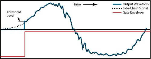
A look-ahead detector works by delaying the main audio signal a short amount (a few millionths of a second) while not delaying the side-chain signal. This allows examining the signal in advance to determine the appropriate response before an event (compare Figure 18 and Figure 19). This action allows the gate (or a ducker) to turn on before the transient signal you want.
Pre-ramping allows gating on the main signal as soon as the signal reaches the threshold. Pre-ramping is sometimes referred to as an exponential envelope since it preserves the overall shape of the original signal.
Combining look-ahead and pre-ramping serves two purposes:
With digital signal processing, it is possible to delay the main signal path as long as desired. The limiting factor is the amount of delay that the application will tolerate. For live sound applications, this threshold is somewhere around two milliseconds, which is equivalent to 96 samples at a 48 kHz sample rate. To accurately reproduce the leading edge of a signal, the function must look-ahead one quarter of a cycle. This means that with a 96 sample look-ahead, a gate can accurately reproduce the leading edge of tones as low as 125 Hz. Look-ahead delays as low as 16 samples (333 microseconds) allow accurate reproduction of signals at or above 750 Hz, and significant improvement in the sound quality of signals as low as 100 Hz. The following bass drum example shows why this is important. Note the difference in amplitude between the first and second cycles of the bass drum. The first complete cycle, and most importantly the leading edge of this cycle, defines the sound.
Even when turned on in time, a gate, by definition, "steps" the gain (see Figures 18 & 19). Unfortunately, gain-steps sound like clicks. Using exponential pre-ramping and look-ahead allows the gate to turn on more gradually, closely simulating the original signal. The click normally associated with gating is gone and the natural sound of the signal is preserved. In postproduction applications, multiple tracks can be time aligned, allowing much longer delays that allow seeing further into the future, thus providing improved low frequency gating.
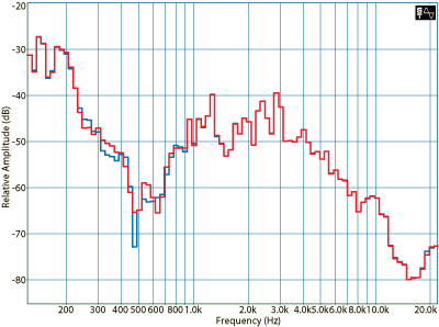
These figures show the affect of look-ahead and pre-ramping on the leading edge of a bass drum. The red trace shows the gate input signal. The blue trace shows the gate output signal. The time difference between the two signals represents the total propagation delay through the gate. The gate threshold is set to about 80% of the peak value. The gate depth is 20 dB.
The first complete cycle of the bass drum defines its sound, as subsequent cycles are considerably lower in amplitude. If the gate cannot accurately capture the first cycle it significantly changes the bass drum's sound.
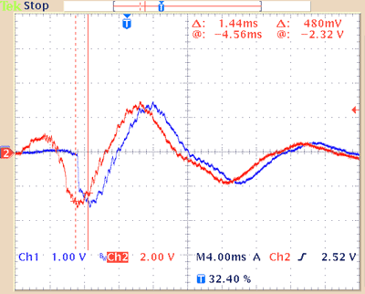
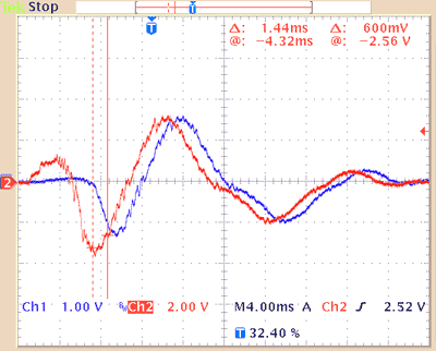
Figure 20 shows look-ahead without ramping which often causes an audible click at fast attack and moderate to extreme depth settings. Only look-ahead with pre-ramping accurately reproduces the first cycle of a bass drum without adding excessive delay or altering the leading edge as shown in Figure 21.
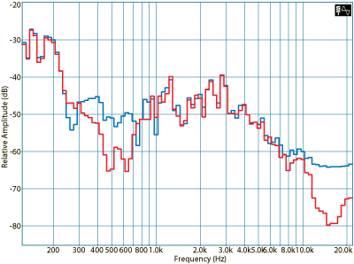
Figures 22 and 23 give the associated frequency response of Figures 20 and 21 respectively. Note in Figure 22 the additional energy above 10 kHz due to the "instant on" nature of a gate without pre-ramping. There is 16 dB of unwanted energy in this region due to the step-like gate opening. Surprising is the 5 dB to 15 dB increase in the 300 Hz to 800 Hz range. Both effects significantly alter the sound of the bass drum.
Compare this with the near-perfect response shown in Figure 23 for a gate with both look-ahead and pre-ramping.
A ducker is a dynamics processor that lowers (ducks) the level of one audio signal based upon the level of a second audio signal or a control trigger. It reduces the level of the main signal by a certain amount (usually labeled Depth) when the side-chain signal exceeds a set threshold.
A typical application is paging. A ducker senses the presence of audio from a paging microphone and triggers a reduction in the output level of the main audio signal for the duration of the page signal. It restores the original level once the page message is over.
Another use is for talkover -- a popular function on DJ mixers that allows the DJ to speak over the program material by triggering a ducker. Also found on recording consoles to allow the producer or engineer to talk to the musicians.
Musical instrument solos use duckers to automatically reduce the bass line a few dB every time the bass drum hits.
Figure 24a shows a typical topology for the ducker. Figure 24b shows the operation of the ducker. A ducker works the opposite of a gate. The signal is attenuated when the side-chain input goes above the threshold. In the example below, the green trace shows the side-chain input. The red trace shows the resulting gain response of the main signal. The threshold is set at -10 dBu. When the side-chain input goes above -10 dBu, the main signal is ducked by an amount set by the depth control, in this case, 40 dB.
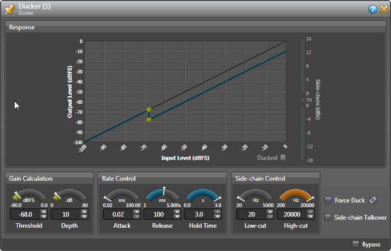
The Hold parameter has a typical range of 0 to 3 seconds. The hold time determines how long the signal remains ducked when the control signal drops below the threshold setting.
A typical Depth control has a range of 0 to -80 dB. The depth control determines how many dB the signal is attenuated when the control signal is at or above the threshold setting.
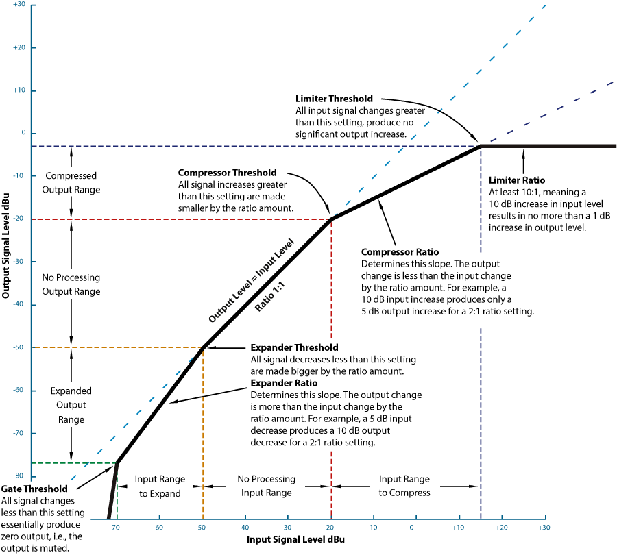
Figure 25 shows how a gate, expander, compressor and limiter all work together on the same program material in a single channel. The vertical axis is the output level and the horizontal axis is the input level.
Setting all ratios at 1:1 makes the input and output of the circuit the same, as illustrated by the straight diagonal line running at 45° across the graph. Whatever comes in goes out unchanged.
Each of the threshold controls acts like a trigger or hinge point, activating gain reduction or expansion only when the input signal exceeds the set point value.
The ratio controls determine how much of an angle the hinge bends, which is how much gain reduction or expansion occurs above or below the threshold. Graphically, the ratio can swing this hinge from 45° (no processing) to almost 90° (full ratio). It is also possible, by adjusting the threshold controls, to have each of these circuits overlap and interact with each other to develop a dynamic curve. The solid black line shows the resultant curve.
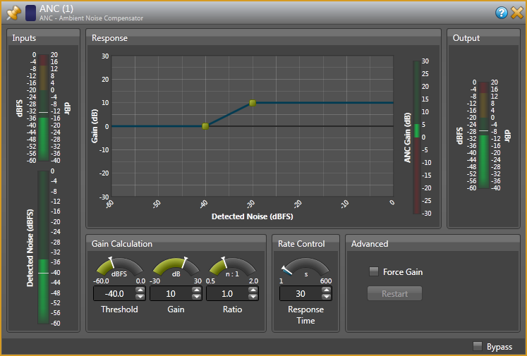
A leveler is a dynamics processor that maintains (levels) the amount of one audio signal based upon the level of a second audio signal. Normally, the second signal is from an ambient noise-sensing microphone. For example, a restaurant or a shopping mall is an application where maintaining paging and background music a specified loudness above the ambient noise is essential. The leveler monitors the background noise, dynamically increasing and decreasing the main audio signal as necessary to maintain a constant loudness differential between the two.
Other names for this function are ambient noise compensation and SPL (sound pressure level) controller.
Acoustic feedback is the phenomenon where the sound from a loudspeaker is picked up by the microphone feeding it, and re-amplified out the same loudspeaker only to return to the same microphone to be re-amplified again, forming an acoustic loop. With each pass, the signal becomes larger until the system runs away and rings or feeds back on itself producing the all-too-common scream or squeal found in sound systems.
These buildups occur at particular frequencies called feedback frequencies.
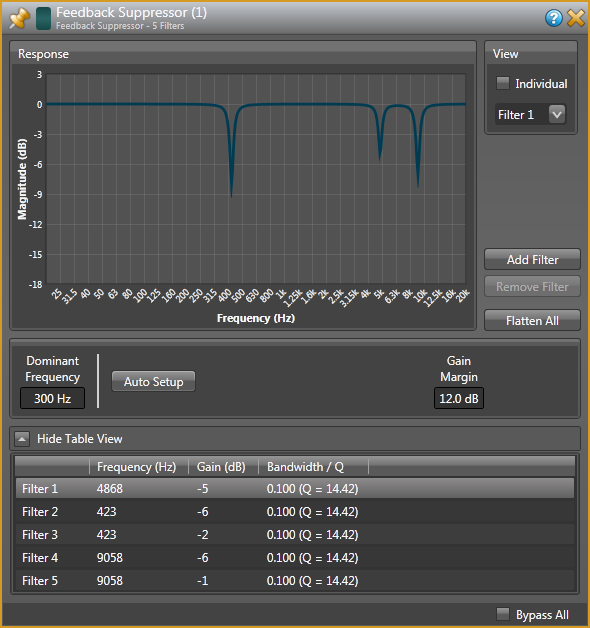
A feedback suppressor is a dynamics processor that uses automatic detection to determine acoustic feedback frequencies and then positions notch filters to cancel the offending frequencies. Other methods use continuous frequency shifting (a very small amount) to prevent frequency build up and feedback before it happens.
Exciters (or enhancers) are any of the popular special effects signal processing products used in both recording and performing. All of them work by adding musical overtones -- harmonic distortion really -- but hopefully pleasing harmonic distortion. For example, tube amps benefit from the harmonic distortion added by their non-linear performance, resulting in a richer, warmer sound. Various means of generating and summing frequency-dependent and amplitude-dependent harmonics exist. Both even- and odd-ordered harmonics find favorite applications. Psychoacoustics teaches that even-harmonics tend to make sounds soft, warm and full, while odd-harmonics tend toward metallic, hollow and bright. Lower-order harmonics control basic timbre, while higher-order harmonics control the edge or bite of the sound. Used with discrimination, harmonic distortion changes the original sound dramatically, more so than measured performance might predict.
Like spice in cooking, a little goes a long way. The problem with heavy compression (low threshold and a high ratio) is the nasty side effects. The timbre of the sound itself changes: it becomes hard and closed, not sweet and open as intended. Breathing and pumping can accompany heavy compression, i.e., the background noise rises way out of proportion to the foreground sound as the compressor releases.
For smoothing level variations between different microphones, use a low compression ratio of 2:1. For line-level averaging, use a higher ratio of 4:1. Initially set the threshold control at 0 dBu, set a ratio of 3:1 and rotate the release control to the middle setting (or auto mode if available) and bring the system level up to 0 dBu (using a recorded source or during rehearsal). Increase the level until the meters respond showing the amount of compression in dB. Experiment with different ratio settings as well as attack and release times (or auto-set mode, if provided).
A tough issue with vocals is the extreme dynamic range of some singers: those who lull you to sleep and then crush you with an unexpected blast. The difference between the soft crooning and the loud climax represents too great a signal change for many preamps and mixers, causing them to clip and distort. For solo vocals the concern is keeping the signal level within the operating range of the equipment -- keeping the quiet parts above the noise floor while keeping the loud parts below the clipping level.
Things get more difficult when the singer in no longer a solo act and has a group of amplified musicians accompanying. The challenge is to keep the vocal(s) prominent while keeping them within a comfortable level compared to the rest of the musicians. If you were to leave the vocal microphones at a high enough gain so that the quiet parts are easily heard, the loud parts might flow forth with far too much level and drown out the rest of the band.
The key is to reduce the vocals dynamic range to something comparable to that of the musicians' instruments. Relatively heavy compression is often used in this scenario, either by using a low ratio (2:1) with a lower threshold (-12 dB) or a higher ratio (4:1) with a higher threshold (-9 dB, or so). Typically set the threshold so that quiet vocal passages show little or no gain reduction and normal singing shows between 3 dB to 6 dB gain reduction when using a 2:1 ratio.
A soft knee characteristic is typically more "musical" sounding with vocals. As an added bonus, a soft knee setting allows using higher ratios since the transition from 1:1 to higher ratios is gradual. This allows the compressor to function more aggressively as the input level rises and you need to clamp down on the signal harder.
Experimentation is the key here; there is no magic setting, but these are good starting points.
When recording vocals use a compressor to reduce the dynamic range of the whole piece to fit the recording or reproduction requirements. Even a small amount of compression makes the whole track sound louder. This increase in perceived loudness results from increasing the average gain by reducing the peaks, i.e., it has a higher average level. This is one of the tricks for bringing the vocals up in any mix, live or recorded.
Good settings for natural sounding, yet compressed vocals, are a medium fast (25 - 50 ms) attack and a medium-slow (100 ms - 1 sec) release. Releasing too quickly sounds unnatural while attacking too slow misses the problem surges.
It is common for the sound mixer to reduce the bass signal because it overwhelms the total system. Use a compressor to smooth a bass sound by lessening the variations between the strings and increasing the sustain.
Typical settings for a bass guitar are a ratio of 4:1, with a fast attack of 25 ms and a slow release of around 500 ms. These settings produce a strong, smooth bass line to start with, and then adjust further as necessary. A hard knee setting is often preferred since all you want is to tame the excessive peaks and leave everything else alone.
Placement of the compressor in the signal chain depends on how you want it to function. For just the input signal, it goes after the bass guitar (if it has a line-level output) and before the preamp. If it is to function as a limiter to protect the speakers in the bass rig, it goes between the preamp and the power amp. Another method is to insert the unit into the effects loop of the preamp. This affects the bass signal by the preamp first, then the compressor limiter, and finally out to the power amp.
Here are a few suggestions on how to achieve a lower volume without sounding as if you are playing out of a transistor radio. Set a slow (~500 ms) attack time with a medium to slow (100 ms – 500 ms) release and a relatively low threshold. Experiment from these initial settings. Do not over compress the high frequencies or the pick attack will sound slurred.
One of the favorite uses of compression by guitarist is to increase the sustain, or duration of a note after it is played. Jeff Beck, Carlos Santana and Gabor Szabo used sustain to great acclaim, although they did it the old-fashioned way of creating feedback by aiming the guitar pick-ups at the loudspeaker and then jamming over it (using a hard limiter to prevent damage). A compressor creates a similar effect. Set a high ratio and low threshold for long sustain, along with fast attack and slow release. Again, experimentation produces the best results.
When using compressors on drums and percussion, it is polar opposite time. Two popular approaches exist for changing the sound character. Both yield pleasant results and allow you to dramatically or subtly change the nature of the sound. Regardless of which approach you try or end up liking, the vast majority of compressor use on drums is limited to snare and bass drum.
The first approach is to use the attack time of the compressor to modify the drum sound. For example, by using a slower attack time along with a 2:1 ratio on a snare drum and by varying the threshold you can make very dramatic changes in the tonal character. By using a slower attack time the initial "crack" of the drum gets through -- great if the drum heads are old. This was a very popular technique for getting a beefy consistent snare sound for many years and is heard on many rock ballads. By only adjusting the attack time and ratio you will be amazed at how many variations of tone are possible, even without a stitch of EQ.
Reducing the leading edge of drum hits is another popular use of compressors. Try ratios between 2:1 and 5:1 accompanied by fast attack and release times. Listen carefully while changing the attack time to find the final setting.
Cymbals need a fast attack but a slow release to allow the sustain through. Begin with a low ratio of 2:1.
Bass drums are difficult to capture consistently due to drumming technique and other issues. It is common to use a compressor to keep the bass drum at a consistent level and tonality. Since many mixes are created with the rhythm section as the foundation, it is important to keep those elements even and consistent. This involves higher ratios (between 4:1 and 10:1) with a fast attack and release time.
To prevent turning the drum sound into pure mush, it is important to use a monitoring system (or the main sound system) having good low frequency performance. Use high ratios to keep the level consistent, and use the fastest attack possible without destroying the drum punch.
Compressors find use primarily on bass guitar, piano, drums and vocals. Another popular application is the drum mix or submix.
For digital recording, use it to compress a too-wide dynamic range into a signal that does not cause digital overload. The limiter is the primary circuit for keeping things under control, but a little compression with its threshold set just under the limiter threshold helps keep the limiting subtle. To control a stereo mix, use the side-chain slave mode.
The following chart shows starting points:
ATTACK |
RELEASE |
RATIO |
KNEE |
|
Vocals |
25 ms to 100 ms |
100 ms to 500 ms |
2:1 to 4:1 |
Soft |
Clicky Bass |
25 ms |
25 ms |
4:1 or higher |
Hard |
Mushy Bass |
100 ms to 500 ms |
100 ms to 500 ms |
4:1 |
Hard |
Raging Electric Guitar |
25 ms |
1 sec - 2 sec |
4:1 or higher (more sustain) |
Hard |
Acoustic Guitar |
100 ms to 500 ms |
100 ms to 500 ms |
4:1 |
Medium |
Brassy Horns |
25 ms |
25 ms |
5:1 or higher |
Hard |
Drums (kick, snare) |
25 ms |
25 ms |
4:1 |
Hard |
Drums (cymbals) |
25 ms |
1 sec - 2 sec |
2:1 to 10:1 |
Hard |
Split-band processing is one of the easiest ways to compress transparently. Broadcast stations use split-band compression regularly, often dividing the spectrum into four or five bands. When it's done right, the radio station sounds great: loud, present, with no squashing or pumping.
The great Dolby noise reduction systems, from Dolby A all the way through B, C, S and SR, all use some variation on compression, expansion and band-splitting.
Split-band techniques work well for several reasons: You can optimize each set of dynamics processors (the compressor, expander and limiter) to a particular range of audio frequencies. That is, the ratio and threshold controls can be suited to each part of the spectrum.
You can decide to process different ranges of an instrument differently. You could use no compression on the low end of a bass, with heavy compression on the top end to put the string slaps in balance with the bottom. Or you could tighten a boomy bottom with compression but leave the top less controlled for an open feeling.
Any massive anomaly like a low frequency breath noise for example, only triggers gain reduction within its range, leaving the desired vocal unaltered. And the decidedly unmusical phenomenon of a popped "p" sucking the overall level back 10 dB is eliminated.
The following tips refer to a compressor design featuring one input with two internal signal paths, each with its own compressor and fed from an adjustable crossover, then summed back together and exiting as one output, as shown here.
A lower stage volume is beneficial in getting a better house mix. Split-processing techniques can achieve a lower volume without sounding tinny.
On-stage big 4 x 12" cabinets create a huge wall of sound, but are often accompanied by an annoying woofing on the low-end. Try setting a crossover point around 400 Hz and compress the bottom-end at a 10:1 ratio. Play a chord where you notice a lot of woofing then set the gain reduction with the threshold control to read 6 dB on the display. If you hit an open chord and there is no gain reduction then it is set right. Compress the top end using a 1.5:1 to 2:1 ratio, along with a 3 dB gain reduction when an open chord is hit. This gives your sound more attack. Play around with these settings. When correct for your instrument, no matter where you play on the neck the bottom-end will sound even, without woofing, giving your overall tone punch and clarity.
Be careful not to over compress the top-end, or the pick attack will slur. If you want more attack, turn up the top-end level.
Solve the problem of overdriving the system by using a split-band compressor to keep the high-end attack, without low-end booming. For more attack, turn up the level on just the high-end.
Begin with a crossover setting of 200 Hz and set the low-end band for mild compression, around 2:1, with the threshold set at -10 dBu. Try setting the high-end band for heavy compression at 6:1, and the threshold at -20 dBu. Turn the volume and the treble controls on the bass full up, and slap and pop hard. You should hear that the high-end is pushed down to the low-end level, yet sounds balanced and not compressed.
Each instrument is different so experiment until pleased with the result. Sometimes slight processing on the lows will tightened the bottom end without sounding controlled or processed. The highs with subtle compression will sound natural without a breathing sound.
Use split-band compression on bass guitar, piano, drums, vocals, anywhere you normally use a compressor. It gives you more control with a less tortured sound. It even sounds good compressing an entire mix.
Of special interest are instruments with large level changes in their different tonal ranges. String pops on a bass are one, but flute is another. The higher tones require more breath and are much louder than the lower.
The split-band approach allows you to apply different amounts of compression to the low- and high-ends of a piano, or you can limit just the high end of the sax.
A split-band compressor does a better job of smoothing the performance out.
Use Dynamic EQ to automatically correct for timbre changes due to the low frequency boost caused by the proximity effect of cardioid microphones (see Figure 28), which occurs when a singer/speaker does not remain a consistent distance from the microphone.
Two opposite applications share this problem:
1. The first occurs when the mic is located far enough from the person that the proximity effect has no bearing (typically a podium situation), then the speaker leans in closer to the microphone causing a low frequency boost.
Start with a 100 to 250 Hz center frequency, a bandwidth of 2.0 octaves and a ratio of 3:1. Set the threshold high enough so that when the person is the normal distance there is no response, and only when they move closer to the mic does the threshold kick the filter into action.
2. The second application compensates for the loss of the proximity effect as the person moves the microphone away from their mouth; typical of most hand held mics.
Solve this problem by perform the opposite routine as the podium mic example above. Have the person hold the microphone at the farthest distance from their mouth that can occur. Set the Dynamic EQ so that it is just below threshold. Once they move the mic closer to their mouth it will reduce the low frequency boost. Since we have become accustomed to hearing the proximity effect try low ratios so that the tonality change is slight, but remains more consistent than without the Dynamic EQ. Use appropriate EQ on the input channel to add back in any missing warmth -- this warms the signal while the Dynamic EQ keeps the tonality consistent.
Typical starting points are a frequency of 100 to 250 Hz, a bandwidth of 2.0 octaves and a ratio of 2:1 depending on the desired change in tonality.
A great example is evening out the tone, or timbre, of a guitar amplifier. Using two channels set up for different tones is very common to switch between a rhythm tone and a lead tone. Often the musician sets the lead tone brighter than the rhythm tone so it cuts through better. The problem comes when the sound system amplifies this all out of proportion, resulting in too much energy around 2 kHz to 4 kHz (a really nasty frequency range due to the ear's maximum sensitivity to this octave).
Setting the Dynamic EQ for a center frequency of 3 kHz and a bandwidth of about 1 octave cleans this up. Set the threshold high enough so that during normal playing nothing is happening. If the device uses relative threshold, once the lead channel is used it will automatically see the change in timbre and apply the Dynamic EQ to reduce the excess energy at 3 kHz relative to the rest of the audio spectrum. You can also use this technique to make guitar sounds "thick" and "chunky" without being overbearing by using the EQ section set in the 200 Hz range as well.
It is common for female singers to have a wide tonality swing when shifting from a quiet breathy passage to a loud crescendo. The voice sounds warm and pleasant during the quiet passage but shows a predominance of frequencies in the 1.2 kHz range for the loud crescendo. This is exaggerated when the singer moves the microphone away from her mouth thereby removing the warming character of the microphone's proximity effect and adds to the naturally occurring peak in this frequency range.
To fix this, simply set the EQ section to the problem frequency (typically 1.2 kHz) and set the threshold so that the compressor only kicks in when she sings the loud passages. Use the ratio control to determine exactly how much of the original tone change remains -- low ratios leave more change while high ratios clamp down hard and allow very little change.
Dynamic EQ lets the user create sounds that change tone with level, or at extreme settings, which allows the creation of radical sounds based on the threshold, attack & release times.
Experiment -- the results will amaze you.
What "compression" is and does has changed significantly over the years. Reducing the dynamic range of the entire signal was the originally use of compressors, but advances in audio technology makes today's compressor use more sparing.
The need for compression arose the very first time anyone tried to record or broadcast audio: the signal exceeded the medium. For example, the sound from a live orchestra easily equals 100 dB dynamic range. Yet early recording and broadcasting medium all suffered from limited dynamic range, e.g., LP record: 65 dB, cassette tape: 60 dB (with noise reduction), analog tape recorder: 70 dB, FM broadcast: 60 dB, AM broadcast: 50 dB. Thus, "6 pounds of audio into a 4 pound bag" beget the compressor.
Early compressors did not have a "threshold" knob; instead, the user set a center ("hinge") point equivalent to the midpoint of the expected dynamic range of the incoming signal. Then a ratio was set which determined the amount of dynamic range reduction. Figure 29 shows that reducing 100 dB to 50 dB requires a 2:1 ratio.
The key to understanding compressors is always to think in terms of increasing and decreasing level changes in dB about the set-point. A compressor makes audio increases and decreases smaller.
From our example, for every input increase of 2 dB above the hinge point the output only increases 1 dB, and for every input decrease of 2 dB below the hinge point the output only decreases 1 dB. If the input increases by x-dB, the output increases by y-dB, and if the input decreases by x-dB, the output decreases by y-dB, where x/y equals the ratio setting. Simple -- but not intuitive and not obvious.
This concept of increasing above the set-point and decreasing below the set-point is where this oft-heard phrase comes from: "compressors make the loud sounds quieter and the quiet sounds louder." If the sound gets louder by 2 dB and the output only increases by 1 dB, then the loud sound is made quieter; and if the sound gets quieter by 2 dB and the output only decreases by 1 dB, then the quiet sound is made louder (it did not decrease as much).
With advances in all aspects of recording, reproduction and broadcasting of audio, the usage of compressors changed from reducing the entire program to just reducing selective portions of the program. Thus was born the threshold control. Now sound engineers set a threshold point such that all audio below this point is unaffected, and all audio above this point is compressed by the amount determined by the ratio control. Therefore the modern usage for compressors is to turn down (or reduce the dynamic range of) just the loudest signals.
Just like compression, what "expansion" is and does has evolved significantly over the years. The original use of expanders was to give the reciprocal function of a compressor, i.e., it undid compression.
Recording or broadcasting audio required compression for optimum transfer. Then it required an expander at the other end to restore the audio to its original dynamic range.
Operating about the same "hinge" point and using the same ratio setting as the compressor, an expander makes audio increases and decreases bigger as diagrammed in Figure 29.
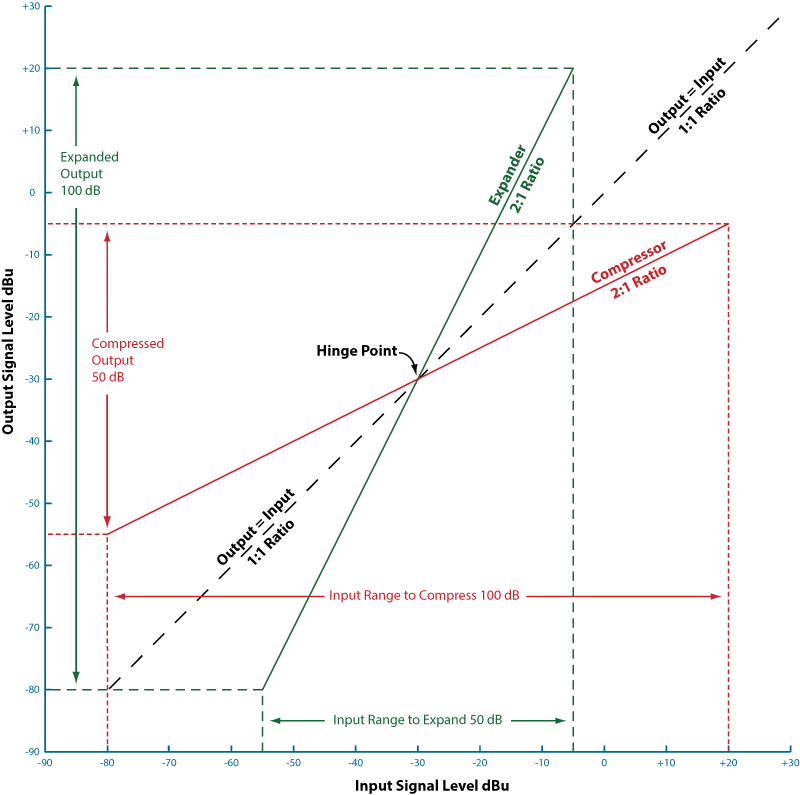
In non-threshold based compressors, a signal is compressed equally above and below a hinge point with the hinge point simply setting a unity gain point. In non-threshold based expanders, the signal is expanded equally above and below a hinge point with the hinge point simply setting a unity gain point.
![]() "Dynamics Processors" This note in PDF.
"Dynamics Processors" This note in PDF.